How To Draw Direction Fields For Differential Equations Matlab

Using Matlab for First Order ODEs

@-functions
Management fields
Numerical solution of initial value problems: Plotting the solution
Combining direction field and solution curves
Finding numerical values at given t values
Symbolic solution of ODEs: Finding the full general solution
Solving initial value problems
Plotting the solution
Finding numerical values at given t values
Symbolic solutions: Dealing with solutions in implicit class

@-functions

Y'all can define a function in Matlab using the @-syntax:

g = @(x) sin(x)*x

defines the role chiliad(x) = sin(x)·ten. You tin and so

evaluate the function for a given x-value:
g(0.3)
plot the graph of the function over an interval:
ezplot(g,[0,20])
discover a zero of the function about an initial judge:
fzero(g,3)

You can also define @-functions of several variables:

G = @(ten,y) 10^4 + y^iv - 4*(x^2+y^2) + four

defines the function G(10,y) = 10^four + y⁴ - iv(10ⁱⁱ + y²) + 4 of two variables. You can then

evaluate the function for given values of ten,y:
G(1,2)
plot the graph of the function as a surface over a rectangle in the x,y airplane:
ezsurf(G,[-2,2,-ii,2])
Click on in the figure toolbar, then you can rotate the graph by dragging with the mouse.
plot the curves where G(ten,y)=0 in a rectangle in the 10,y plane:
ezplot(G,[-ii,two,-2,2])
make a contour plot of the function for a rectangle in the x,y aeroplane:
ezcontour(G,[-ii,2,-ii,2]); colorbar

Direction Fields

Offset download the file dirfield.m and put it in the same directory as your other m-files for the homework.

Define an @-function f of 2 variables t, y corresponding to the right hand side of the differential equation y'(t) = f(t,y(t)). East.g., for the differential equation y'(t) = t y ² ascertain

f = @(t,y) t*y^2

You must use @(t,y)..., even if t or y does not occur in your formula.
E.g., for the ODE y'=y² you would use f=@(t,y)y^2

To plot the management field for t going from t0 to t1 with a spacing of dt and y going from y0 to y1 with a spacing of dy use dirfield(f,t0:dt:t1,y0:dy:y1) . East.thou., for t and y between -2 and 2 with a spacing of 0.2 type

dirfield(f,-2:0.2:ii,-2:0.2:2)

Solving an initial value problem numerically

First define the @-role f corresponding to the correct hand side of the differential equation y'(t) = f(t,y(t)). E.g., for the differential equation y'(t) = t y ² define

f = @(t,y) t*y^2

To plot the numerical solution of an initial value problem: For the initial condition y(t0)=y0 you lot tin plot the solution for t going from t0 to t1 using ode45(f,[t0,t1],y0) .

Example: To plot the solution of the initial value problem y'(t) = t y ², y(-ii)=1 in the interval [-2,2] use

[ts,ys] = ode45(f,[-two,two],1) plot(ts,ys,'o-')

The circles mark the values which were actually computed (the points are called by Matlab to optimize accuracy and efficiency). The vectors ts and ys contain the coordinates of these points, to see them equally a table blazon [ts,ys]

You can plot the solution without the circles using plot(ts,ys) .

To combine plots of the direction field and several solution curves use the commands hold on and hold off : Later obtaining the first plot type concord on, then all subsequent commands plot in the same window. Afterwards the final plot command type hold off.

Example: Plot the direction field and the 13 solution curves with the initial conditions y(-2) = -0.4, -0.2, ..., one.viii, 2:

dirfield(f,-2:0.two:ii,-2:0.2:two) hold on  for y0=-0.4:0.2:2    [ts,ys] = ode45(f,[-2,2],y0); plot(ts,ys)  end  hold off

To obtain numerical values of the solution at certain t values: You can specify a vector tv of t values and utilize [ts,ys] = ode45(g,television,y0) . The first element of the vector tv is the initial t value; the vector television receiver must take at to the lowest degree 3 elements. East.g., to obtain the solution with the initial status y(-2)=1 at t = -2, -1.v, ..., 1.5, two and display the results as a table with two columns, employ

[ts,ys]=ode45(f,-2:0.five:ii,1); [ts,ys]

To obtain the numerical value of the solution at the terminal t-value use ys(end) .

Information technology may happen that the solution does not exist on the whole interval:

f = @(t,y) t*y^2 [ts,ys] = ode45(f,[0,ii],2);

In this example ode45 prints a warning "Failure at t=..." to show where information technology stopped.

Annotation that in some cases ode15s performs better than ode45. This happens for so-called strong problems. ode15s is also better at detecting where a solution stops to exist if the gradient becomes space.

Solving a differential equation symbolically

You have to specify the differential equation in a cord, using Dy for y'(t) and y for y(t): E.k., for the differential equation y'(t) = t y ^two type

sol = dsolve('Dy=t*y^2','t')

The last argument 't' is the name of the independent variable. Practise not type y(t) instead of y.

If Matlab tin can't detect a solution it will return an empty symbol. If Matlab finds several solutions information technology returns a vector of solutions.

Here there are two solutions and Matlab returns a vector sol with 2 components: sol(one) is 0 and sol(ii) is -ane/(t^ii/two + C3) with an capricious constant C3.

The solution volition contain a constant C3 (or C4,C5 etc.). You tin can substitute values for the constant using subs(sol,'C3',value) . Due east.g., to set C3 in sol(2) to 5 utilise

subs(sol(2),'C3',5)

To solve an initial value problem additionally specify an initial condition:

sol = dsolve('Dy=t*y^ii','y(-2)=one','t')

To plot the solution apply ezplot(sol,[t0,t1]) . Here is an example for plotting the solution curve with the initial conditions y(-2) = -0.4:

sol = dsolve('Dy=t*y^2','y(-2)=-0.4','t') ezplot( sol , [-two ii])

To obtain numerical values at one or more than t values apply subs(sol,'t',tval) and double (or vpa for more digits):

sol = dsolve('Dy=t*y^2','y(-2)=1','t')

This gives a numerical value of the solution at t=0.5:

double( subs(sol,'t',0.v) )

This computes numerical values of the solution at t=-2, -1.five, ..., 2 and displays the consequence as a tabular array with two columns:

tval = (-2:0.five:2)'; % column vector with t-values yval = double( subs(sol,'t',tval) )% column vector with y-values [tval,yval] % display ii columns together

Symbolic solutions: Dealing with solutions in implicit form

Ofttimes dsolve says 'Explicit solution could not exist found'. But in many cases ane can still obtain the solution in implicit form, and utilise this to plot the graph of the solution, or to obtain numerical approximations.

If dsolve says 'Explicit solution could not exist found' in that location are two possibilities: (Note that different versions of the symbolic toolbox comport differently)

dsolve returns the answer in the form RootOf(expression,z) or solve(equation,y)
Example 1: Solve the IVP y'=t/(y^iv-1), y(ane)=0.
dsolve('Dy=t/(y^4-ane),y(1)=0','t')
returns in Matlab R2010b
RootOf(X89^5 - five*X89 - (five*t^two)/2 + 5/2, X89)
This means that the solution in implicit form is
y^five - 5y - 5t²/ii + 5/two = 0
dsolve returns the respond [ empty sym ]
In this case Matlab was unable to observe the solution in implicit form. In older versions (e.g. Matlab R2010b) this can even happen when it like shooting fish in a barrel to find by hand the solution in implicit form. In some cases omitting the initial status helps:
For Example 1 newer Matlab versions (R2011b, R2012b) return [empty sym]. In this case using dsolve('Dy=t/(y^four-1)','t') gives the implicit solution with a abiding. Nosotros tin so find the value of the constant using the initial condition.

Plotting the solution of IVP in implicit form: If the solution in implicit class is expression=0 apply
ezplot(expression,[ t_min t_max y_min y_min ])
to plot the solution y(t) for t_min ≤ t ≤ t_max, y_min ≤ y ≤ y_max.
E.g., for Example i we can plot the initial indicate together with the solution curve by
hold on; plot(1,0,'o'); ezplot('y^5 - 5*y + 5/2 - 5*t^2/2',[-two 2 -2 2]); filigree on; hold off

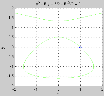
Nosotros see from the graph that the interval where the solution exists is roughly (-1.6, 1.half-dozen).

Plotting the general solution in implicit form: If the general solution in implicit grade is expression=C with C capricious, utilize
ezcontour(expression,[ t_min t_max y_min y_min ])
Due east.g., for Instance 1 we tin plot the general solution past
ezcontour('y^5 - 5*y + 5/2 - 5*t^2/two',[-two two -2 2])
ezcontour plots contours for 9 values of C. If you lot want to see more contour curves: Download the file ezcontourc.m and put it in the aforementioned directory equally your other m-files. Then you tin can apply e.g.
ezcontourc('y^five - 5*y + five/2 - five*t^2/two',[-2 2 -2 2],fifty)
to obtain contour curves for 50 values of C.

Finding values of the solution in implicit form:
For Example 1 we obtained the solution in implicit form y^five - 5y + 5/2 - 5t²/2 = 0.
We now want to find y(1.5): Nosotros plug t=1.5 into the equation and demand to solve the equation y⁵ - 5y + 5/two - 5·one.5ⁱⁱ/2 = 0 for y. From the graph above we can meet that there are actually 3 solutions: near -1.5, near -0.5, and almost i.five. The solution we desire is the ane almost -0.v.

To find a solution y near -0.5 utilize
t=1.v; fzero(@(y)y^5-5*y+5/2-five*t^2/2,-0.5)
which returns the answer y=-0.647819.

Tobias von Petersdorff